Customer Segmentation through KMeans Clustering
This page is still a work in progress and I was having some trouble converting from .ipynb files. Check back later for the completed page.
Importing and Cleaning Data
# import general packages
%matplotlib inline
import numpy as np
import pandas as pd
import matplotlib.pyplot as plt
import seaborn as sns
sns.set()
# loading data and renaming columns
# data comes from a professor of mine and is likely simulated
shopping_data = pd.read_csv('https://raw.githubusercontent.com/zariable/data/master/shopping_data.csv')
shopping_data.rename(
    columns={
        'CustomerID': 'customer_id',
        'Genre': 'genre',
        'Age': 'age',
        'Annual Income (k$)': 'annual_income',
        'Spending Score (1-100)': 'spending_score'
    },
    inplace=True
)
print("Original Dataset")
display(shopping_data.head())

# retain only annual_income and spending_score for 2-D clustering
X = shopping_data.iloc[:,3:5]
print("\n\nTruncated Dataset")
display(X.head())
Original Dataset
| customer_id | genre | age | annual_income | spending_score | |
|---|---|---|---|---|---|
| 0 | 1 | Male | 19 | 15 | 39 |
| 1 | 2 | Male | 21 | 15 | 81 |
| 2 | 3 | Female | 20 | 16 | 6 |
| 3 | 4 | Female | 23 | 16 | 77 |
| 4 | 5 | Female | 31 | 17 | 40 |
Truncated Dataset
| annual_income | spending_score | |
|---|---|---|
| 0 | 15 | 39 |
| 1 | 15 | 81 |
| 2 | 16 | 6 |
| 3 | 16 | 77 |
| 4 | 17 | 40 |
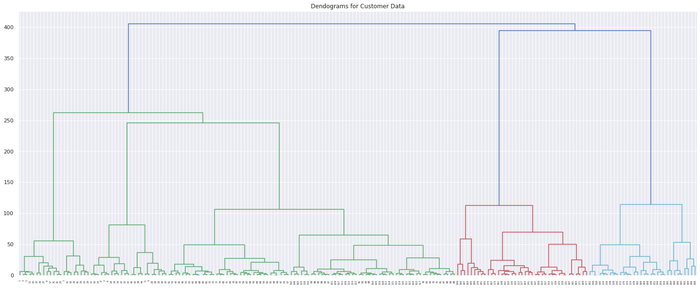
Hierarchical Clustering through Dendogram
import scipy.cluster.hierarchy as shc

# create dendogram to visualize data
plt.figure(figsize=(25, 10))
plt.title("Dendogram for Customer Data")
dend = shc.dendrogram(shc.linkage(X, method='ward'))
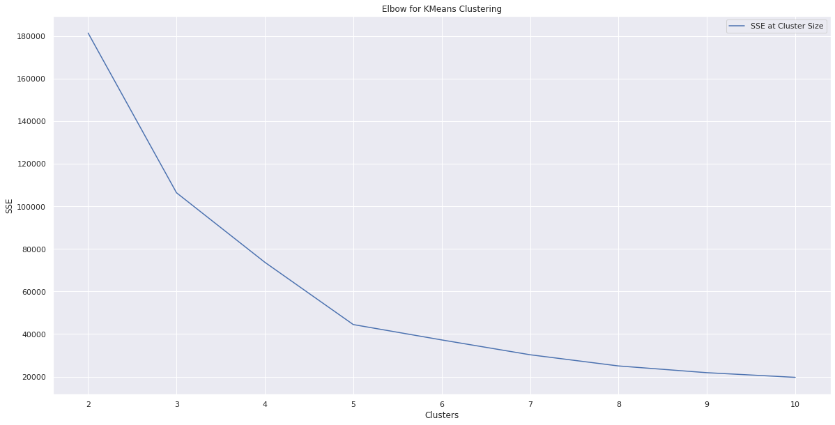
K-means Clustering with SSE
from sklearn.cluster import KMeans

k_range = range(2,11)
sse = []
for k in k_range:
  clusterer = KMeans(n_clusters=k, random_state=0)
  cluster_lables = clusterer.fit_predict(X)
  sse.append(clusterer.inertia_)
fig = plt.figure(figsize=(20,10))
plt.plot(k_range, sse, label = "SSE at Cluster Size")
plt.xlabel("Clusters")
plt.ylabel("SSE")
plt.title("Elbow for KMeans Clustering")
plt.legend()
plt.show()

# k = 5 covers most of the variance with diminishing returns at k > 5
Exploring Different Cluster Sizes
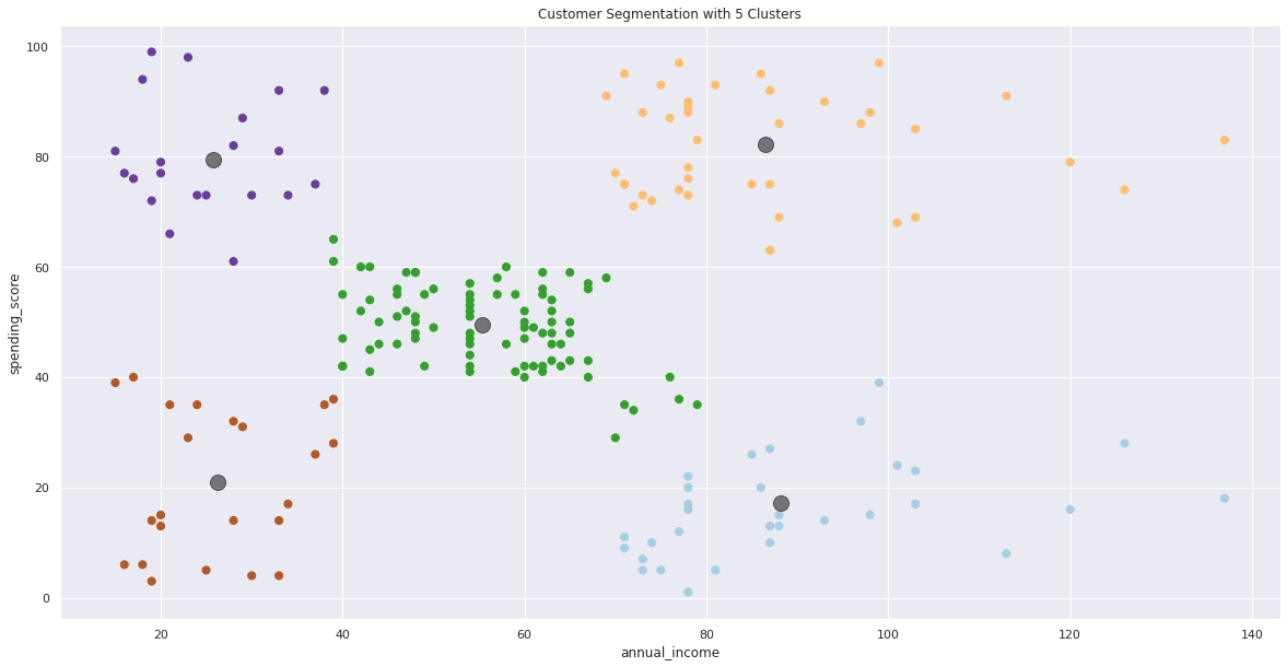
5 Clusters
# generating predictions and showing values based on cluster size

from sklearn.cluster import KMeans
kmeans = KMeans(n_clusters=5)
kmeans.fit(X)
y_kmeans = kmeans.predict(X)
print('Predictions\n\n',y_kmeans,"\n\n\nFrequency of Prediction Labels\n")

unique, counts = np.unique(y_kmeans, return_counts=True)
frequency=pd.DataFrame(zip(unique, counts))
frequency[1]
Predictions

 [4 0 4 0 4 0 4 0 4 0 4 0 4 0 4 0 4 0 4 0 4 0 4 0 4 0 4 0 4 0 4 0 4 0 4 0 4
 0 4 0 4 0 4 2 4 0 2 2 2 2 2 2 2 2 2 2 2 2 2 2 2 2 2 2 2 2 2 2 2 2 2 2 2 2
 2 2 2 2 2 2 2 2 2 2 2 2 2 2 2 2 2 2 2 2 2 2 2 2 2 2 2 2 2 2 2 2 2 2 2 2 2
 2 2 2 2 2 2 2 2 2 2 2 2 3 1 3 2 3 1 3 1 3 2 3 1 3 1 3 1 3 1 3 2 3 1 3 1 3
 1 3 1 3 1 3 1 3 1 3 1 3 1 3 1 3 1 3 1 3 1 3 1 3 1 3 1 3 1 3 1 3 1 3 1 3 1
 3 1 3 1 3 1 3 1 3 1 3 1 3 1 3]


Frequency of Prediction Labels

0    22
1    35
2    81
3    39
4    23
Name: 1, dtype: int64
# generating scatter plot for predictions

from sklearn.cluster import AgglomerativeClustering

hc = AgglomerativeClustering(n_clusters=5, affinity='euclidean', linkage='ward')
y_ward = hc.fit_predict(X)

plt.figure(figsize=(20, 10))
plt.scatter(X.iloc[:, 0], X.iloc[:, 1], c=y_ward, cmap='Paired', s=50)
plt.title('Customer Segmentation with 5 Clusters')
plt.xlabel(X.columns[0])
plt.ylabel(X.columns[1])

centers = kmeans.cluster_centers_
plt.scatter(centers[:, 0], centers[:, 1], c='black', s=200, alpha=0.5)
8 Clusters
# generating predictions and showing values based on cluster size

from sklearn.cluster import KMeans
kmeans = KMeans(n_clusters=8)
kmeans.fit(X)
y_kmeans = kmeans.predict(X)
print('Predictions\n\n',y_kmeans,"\n\n\nFrequency of Prediction Labels\n")

unique, counts = np.unique(y_kmeans, return_counts=True)
frequency=pd.DataFrame(zip(unique, counts))
frequency[1]
Predictions

 [4 3 4 3 4 3 4 3 4 3 4 3 4 3 4 3 4 3 4 3 4 3 4 3 4 3 4 3 4 3 4 3 4 3 4 3 4
 3 4 3 1 3 1 1 4 1 1 1 1 1 1 1 1 1 1 1 1 1 1 1 1 1 1 1 1 1 1 1 1 1 1 1 1 1
 1 1 1 1 1 1 1 1 1 1 1 1 1 1 1 7 7 7 7 7 7 7 7 7 7 7 7 7 7 7 7 7 7 7 7 7 7
 7 7 7 7 7 7 7 7 7 7 7 7 0 7 0 7 0 2 0 2 0 7 0 2 0 2 0 2 0 2 0 7 0 2 0 7 0
 2 0 2 0 2 0 2 0 2 0 2 0 7 0 2 0 2 0 2 0 2 0 2 0 2 0 2 0 2 0 2 0 6 0 6 0 6
 0 6 5 6 5 6 5 6 5 6 5 6 5 6 5]


Frequency of Prediction Labels

0    32
1    47
2    22
3    21
4    21
5     7
6    10
7    40
Name: 1, dtype: int64
# generating scatter plot for predictions

from sklearn.cluster import AgglomerativeClustering

hc = AgglomerativeClustering(n_clusters=8, affinity='euclidean', linkage='ward')
y_ward = hc.fit_predict(X)

plt.figure(figsize=(20, 10))
plt.scatter(X.iloc[:, 0], X.iloc[:, 1], c=y_ward, cmap='Paired', s=50)
plt.title('Customer Segmentation with 8 Clusters')
plt.xlabel(X.columns[0])
plt.ylabel(X.columns[1])

centers = kmeans.cluster_centers_
plt.scatter(centers[:, 0], centers[:, 1], c='black', s=200, alpha=0.5)
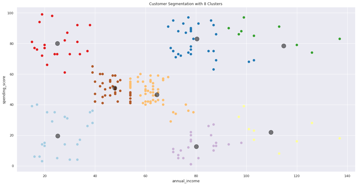
Results
placeholder
basically 5 clusters is better than 8 clusters